---
title: Building an MLB Rating Model
date: last-modified
format:
html:
code-fold: show
code-tools: true
toc: true
code-annotations: below
fig-width: 8
fig-height: 6
fit-dpi: retina
fig-responsive: true
embed-resources: false
params:
season: 2026
execute:
warning: false
---
```{r setup}
#| code-fold: true
#| code-summary: "Setup code"
suppressPackageStartupMessages({
  library(cmdstanr)
  library(posterior)
  library(tidybayes)
  library(geomtextpath)
  library(scales)
  library(gt)
  library(here)
  library(tidyverse)

  devtools::load_all()
})

season <- params$season

knitr::knit_hooks$set(inline = function(x) {
  if (is.numeric(x)) comma(x) else x
})
```
# The Model
To generate team ratings, we'll use a dynamic Bradley-Terry model with covariates.
Like all rating models, a Bradley-Terry model attempts to predict the winner of a head-to-head matchup between two teams on the basis of a numerical rating specific to each team.
## Basic model
A basic Bradley-Terry model assumes each team's rating is a single number, and that the odds of a team winning are equal to the ratio of their ratings: $$
\require{physics}
\frac{\Pr(\text{A wins})}{\Pr(\text{B wins})} = \frac{\exp(\theta_A)}{\exp(\theta_B)}, \qq{so}
\log \frac{\Pr(\text{A wins})}{\Pr(\text{B wins})} = \theta_A - \theta_B,
$$ where the log ratings are denoted by $\theta$.
This is just a logistic regression model with coefficients for each team; the coefficients enter with positive sign for the home team and negative sign for the away team.
In other words, if game $i$ is played between team $\text{home}[i]$ and $\text{away}[i]$, the probability the home team wins, $p_i$, satisfies $$
\mathrm{logit}(p_i) = \theta_{\text{home}[i]} - \theta_{\text{away}[i]}.
$$
This model can be then straightforwardly extended to include covariates (like travel or rest), which are added to the linear predictor above as $X\beta$.
An intercept term corresponds to a home-field advantage, since it uniformly increases the probability the home team wins.
## Adding time
To make this basic Bradley-Terry model *dynamic*, we replace the fixed team ratings with time-varying ratings.
The main part of the model is then $$
\mathrm{logit}(p_i) = \theta_{\text{home}[i], t[i]} - \theta_{\text{away}[i],t[i]} + \vec x_i\beta,
$$ for a game played at time $t[i]$.
We then must specify a time series model for how the (latent) team ratings evolve.
We'll go with a simple AR(1) process: for every team $j$ and time $t>1$, $$
\theta_{j, t} = \theta^*_j + \rho (\theta_{j, t-1}-\theta^*_j) + \epsilon_{jt},
\qquad \epsilon_{jt} \stackrel{iid}{\sim} \mathcal{N}(0, \tilde\sigma^2),
$$ with a prior placed on the first rating for each team $\theta_{j,1}$.
The model is completed by placing priors on the remaining parameters.
## Using splines
We'll want ratings for every day of the season, but that doesn't necessarily mean we want a rating parameter for each team and day---we just don't expect team ratings to vary much on that kind of short timescale.
So we'll simplify the model computationally by making the AR(1) process govern not the ratings directly, but rather knots for a spline basis in time, from which the ratings will be derived.
So if there are $D$ days and $K$ time knots, and we have a $D$-by-$K$ matrix $B$ containing the spline basis, then our model is \begin{align}
z_{j, k} &= z^*_j + \rho (z_{j, k-1}-z^*_j) + \epsilon_{jk},
\qquad \epsilon_{jk} \stackrel{iid}{\sim} \mathcal{N}(0, \tilde\sigma^2), \\
\vec\theta_j &= B\vec z_j,
\end{align} for team $j$ and knot index $k$.
# Calibrating the model to past seasons
We'll fit the model to data from the past ten MLB seasons, excluding 2020.
This will let us pin down $\beta$, $\rho$, and $\tilde\sigma^2$ for use in ongoing and future seasons.
The table below shows a sample of games.
The column `result` is 1 if the home team wins.
```{r}
seasons <- setdiff(2012:(season - 1), 2020)

if (!file.exists(path <- here("data/retrosheet_historical.rds"))) {
  d <- map(sort(seasons), game_data_retro) |>
    setNames(seasons) |>
    bind_rows()
  write_rds(d, path, compress = "xz")
} else {
  d <- read_rds(path)
}

historical_season <- max(d$season, na.rm = TRUE)

slice_sample(d, n = 7) |>
  knitr::kable()
```
The other advantage of fitting to multiple past seasons is that we can learn how to build an informative prior for each team's start-of-season rating, based on their rating at the end of the previous season.
Specifically, we can add one final component to the model, for a season numbered $s>1$: $$
z^*_{s,j} \sim \mathcal{N}(\alpha\,z^*_{s-1,j}, \tau^2),
$$ so that the average rating for season $s$ is centered at the previous season's average rating, but mean-reverted according to $\alpha$.
The parameter $\tau$ controls how confident we are in these prior guesses for teams' ratings.
## Building the model in Stan
{height="3em" fig-align="center"}
The data block is straightforward: we define the dimensions of the problem, and provide indexing vectors for season, day of the seasons, and home and away teams, as well as the vector with the game results.
We also provide the covariate matrix, the spline basis; `knot_space`, which is how many days apart the spline knots are spaced; and a bunch of control parameters to easily specify our priors.
``` stan
data {
  int<lower=2> T; // teams
  int<lower=1> N; // games
  int<lower=1> D; // maximum days
  int<lower=2> K; // knots
  int<lower=1> S; // seasons
  int<lower=1> P; // covariates

  array[N] int<lower=1, upper=D> day;
  array[N] int<lower=1, upper=S> season;
  array[S] int<lower=1, upper=D> n_days; // actual days per season
  array[N] int<lower=1, upper=T> home;
  array[N] int<lower=1, upper=T> away;
  array[N] int<lower=0, upper=1> result;
  matrix[N, P] X; // covariate matrix

  real<lower=1> knot_space;
  matrix[D, K] splines;

  vector[T] prior_rate_loc;
  vector<lower=0>[T] prior_rate_scale;
  vector<lower=0>[2] prior_rho;
  real<lower=0> prior_sigma_scale;
  real<lower=0> prior_sigma_shape;
  real<lower=0> prior_beta_scale;
  real<lower=1> prior_beta_df;
  real prior_alpha_loc;
  real<lower=0> prior_alpha_scale;
  real<lower=0> prior_tau_scale;
  real<lower=0> prior_tau_shape;
}
```
Next we declare the model's raw parameters.
These are mostly straightforward, with a few exceptions annotated below.
<!-- Click on each annotation to see the explanation. -->
``` stan
parameters {
array[S] vector[T] z_loc; # <1>
array[S, T] vector[K] z_knots; # <2>
vector[P] beta;
real alpha; // regression between seasons
real<lower=0> tau10; // s.d. for new season # <3>
real<lower=0, upper=1> rho;
real<lower=0> sigma10; # <4>
}
```
1. `z_loc` is used in a *non-centered parametrization* of $\theta^*_j$, each team's mean rating for the season.
2. `z_knots` are used in a non-centered parametrization of the AR(1) process.
3. `tau10` is $10\times\tau$.
The factor of 10 is cancelled later, but helps with computational speed and stability.
4. `sigma10` is $10\times\sigma$ (not $\tilde\sigma$!).
The difference between $\sigma$ and $\tilde\sigma$ is that the former controls the variance of the whole AR(1) process, while the latter controls the variance of error terms within the process.
Before we can define the model, we need to map the raw `z_knots` parameter into a set of actual team ratings.
This happens in the transformed parameters block.
The Stan code is a bit messy due to the non-centered parametrization (explained below) and the need to vectorize as much of the specification as possible.
Several annotations are provided to make it all clearer.
``` stan
transformed data {
vector[K-1] rho_expo = knot_space * reverse(linspaced_vector(K-1, 1, K-1)) / 7.0; # <1>
}
transformed parameters {
array[S, T] vector[D] ratings;
array[S] vector[T] rate_loc;
real sigma_sc = 0.1 * sigma10 * sqrt(1 - rho^(knot_space / 3.5)); # <2>
vector[K-1] rho_vec = rho^rho_expo; # <3>
// first season
for (t in 1:T) { # <4>
vector[K] raw;
rate_loc[1, t] = prior_rate_loc[t] + prior_rate_scale[t] * z_loc[1, t];
raw[1] = rate_loc[1, t] + 0.1*sigma10 * z_knots[1, t, 1]; # <5>
raw[2:K] = rate_loc[1, t] + reverse(rho_vec) * (raw[1] - rate_loc[1, t]) + # <6>
sigma_sc * cumulative_sum(rho_vec .* z_knots[1, t, 2:K]) ./ rho_vec; # <6>
ratings[1, t] = splines * raw; # <7>
}
// subsequent seasons
for (s in 2:S) {
for (t in 1:T) {
vector[K] raw;
rate_loc[s, t] = alpha*rate_loc[s - 1, t] + 0.1*tau10 * z_loc[s, t]; #<8>
raw[1] = rate_loc[s, t] + 0.1*sigma10 * z_knots[s, t, 1];
raw[2:K] = rate_loc[s, t] + reverse(rho_vec) * (raw[1] - rate_loc[s, t]) +
sigma_sc * cumulative_sum(rho_vec .* z_knots[s, t, 2:K]) ./ rho_vec;
ratings[s, t] = splines * raw;
}
}
}
```
1. We pre-compute a vector of exponents which is used later.
2. This maps `sigma10`, which controls the variance of the whole AR(1) process, to our parameter $\tilde\sigma$, which scales the AR(1) error terms.
3. This creates a vector like $(\rho, \rho^2, \rho^3, \dots, \rho^K)$, but with the exponents rescaled by `knot_space` so that we can interpret $\rho$ on a per-day basis, independent of how the knots are spaced.
4. We specify the AR(1) process for each team, one at a time.
5. The prior on a team's rating in the first season is Normal, with mean and variance provided by the model user.
We can write that here as a location shift `prior_rate_loc[t]` plus a scale (std. deviation) `prior_rate_scale[t]` times a parameter `z_knots[1, t, 1]` which has a $\mathcal{N}(0, 1)$ prior.
This is the simplest version of what's called a *non-centered parametrization*.
6. The AR(1) equation is $z_k=z^* + \rho (z_{k-1}-z^*) + \epsilon_k$ (dropping the team subscript).
By substituting in the same equation for $z_{k-1}$, and then for $z_{k-2}$, and so on, we can find that $$
z_k=z^* + \rho^{k-1}(z_1 - z^*) + \sum_{l=0}^{k-2} \rho^l\epsilon_{k-l}.
$$
We can express $\epsilon_{k-l}$ as $\tilde\sigma$ times a standard Normal variable.
Then the code highlighted here implements this re-expressed equation in vectorized form.
This re-expression is helpful because it makes the $z_k$ uncorrelated with each other in the posterior, as well as uncorrelated with $z^*$, $\tilde\sigma$, and $\rho$.
7. Here is where we apply the spline basis to come up with the actual day-by-day ratings for the team.
8. This line implements the pre-season ratings prior based on the previous season's ratings.
Finally, we implement the core of the model itself.
Several more annotations are provided.
``` stan
model {
vector[N] rate_diff;
for (i in 1:N) {
rate_diff[i] = ratings[season[i], home[i], day[i]] - # <1>
ratings[season[i], away[i], day[i]]; # <1>
}
result ~ bernoulli_logit(rate_diff + X*beta); # <2>
for (s in 1:S) { # <3>
z_loc[s] ~ std_norma(); # should this be std_normal()?
for (t in 1:T) {
z_knots[s, t] ~ std_normal();
}
}
beta ~ student_t(prior_beta_df, 0, prior_beta_scale);
alpha ~ normal(prior_alpha_loc, prior_alpha_scale);
tau10 ~ gamma(prior_tau_shape, 0.1 * prior_tau_shape/prior_tau_scale);
rho ~ beta(prior_rho[1], prior_rho[2]);
sigma10 ~ gamma(prior_sigma_shape, 0.1 * prior_sigma_shape/prior_sigma_scale);
}
```
1. We look up the log-ratings difference between the teams playing each game in the array of season-team-day ratings.
2. The actual likelihood.
The covariate adjustment is added to the ratings difference.
3. Priors for all the parameters.
Notice the raw `z_knots` variable receives a standard Normal prior.
This is part of the non-centered parametrization.
All of the actual work with this variable is done above, in the transformed parameters block.
## Fitting the model
We're now ready to fit the model to the `r nrow(d)` games we have.
We first need a function to create a `list()` with our games in the model's data format.
We'll allow this function to vary how far apart the spline basis knots are spaced in time.
```{r}
#| code-fold: true
#| code-summary: "Data prep code"
form <- ~ 1 + rest_0_home + rest_2_home + rest_2_away + I(rest_3p_home + rest_3p_away)
prep_data_multi <- function(d, knot_space = 7) {
  max_days <- max(d$day)
  m_spline <- splines::bs(seq_len(max_days),
    df = round(max_days / knot_space),
    degree = 1, intercept = TRUE
  )
  n_teams <- nlevels(d$home)
  season <- as.factor(d$season)
  X <- model.matrix(form, d)

  list(
    `T` = n_teams,
    N = nrow(d),
    S = nlevels(season),
    D = max_days,
    K = ncol(m_spline),
    P = ncol(X),
    day = d$day,
    season = as.integer(season),
    n_days = tapply(d$day, season, max),
    home = as.integer(d$home),
    away = as.integer(d$away),
    result = as.integer(d$result),
    X = X,
    knot_space = knot_space,
    splines = m_spline,
    prior_rate_loc = rep(0, n_teams),
    prior_rate_scale = rep(0.5, n_teams),
    prior_rho = c(8, 4),
    prior_sigma_scale = 0.4,
    prior_sigma_shape = 3.0,
    prior_beta_scale = 2.5,
    prior_beta_df = 5,
    prior_alpha_loc = 0.5,
    prior_alpha_scale = 0.7,
    prior_tau_scale = 0.5,
    prior_tau_shape = 2.0
  )
}
```
Then we can compile the Stan model and fit it!
We'll space knots every three weeks to start, and include the following covariates:
- A constant intercept, representing home-field advantage
- Indicators for whether the home and away team have received 0, 2, or 3+ days of rest (0 being a double-header day).
```{r fit-multi}
hyperpars <- c("beta", "alpha", "tau10", "rho", "sigma10")
if (!file.exists(path <- here("data/fit_historical.rds"))) {
  sm <- cmdstan_model(here("R/stan/ratings_multi.stan"), stanc_options = list("O1"))

  fit <- sm$sample(
    data = prep_data_multi(d, knot_space = 21),
    chains = 4, iter_warmup = 800, iter_sampling = 400, thin = 2,
    refresh = 50, adapt_delta = 0.85, step_size = 0.15
  )
  draws <- fit$draws(c(hyperpars, "ratings"))
  nms <- dimnames(draws)$variable
  rgx <- str_glue("({str_c(hyperpars, collapse='|')}|ratings\\[10,)")
  draws <- draws[, , str_starts(nms, rgx)]
  dimnames(draws)$variable <- str_replace(dimnames(draws)$variable, "ratings\\[10,", "ratings[")
  write_rds(draws, path, compress = "xz")
} else {
  draws <- read_rds(path)
}

idx_rate <- which(str_starts(dimnames(draws)$variable, "ratings\\["))
d_sum <- summary(draws[, , -idx_rate])
rv_rate <- as_draws_rvars(draws[, , idx_rate])$ratings[, 182, drop = TRUE]
names(rv_rate) <- d_teams$abbr

knitr::kable(d_sum)
```
We can interpret these hyperparameters as follows:
- $\beta_1$ (the intercept) is estimated at `r number(d_sum$median[1], 0.01)`, so home-field advantage confers about a 15% increase in the odds of winning (like moving an even-odds game to a 53.5% win probability) when both teams are typically rested.
- $\alpha$ is estimated at `r number(d_sum$median[2], 0.01)`, so there's about an 70% correlation between a team's average ratings in back-to-back seasons.
- $\tau$ is estimated at `r number(d_sum$median[3]/10, 0.01)` (remember the factor of 10), so we are reasonably confident about this new season rating.
- $\rho$ is estimated at `r number(d_sum$median[4], 0.001)`, meaning that team's ratings week-to-week are about 80% correlated.
However, the posterior for $\rho$ is extremely close to its prior, meaning that the data are not very informative about this parameter.
Consequently, we will fix $\rho$ to one value in our single-season model, and take it as an additional modeling assumption.
- $\sigma$ is estimated at `r number(d_sum$median[5]/10, 0.01)`, capturing the standard deviation of team ratings.
In other words, we'd expect a team's rating to vary on the order of 10% over the course of a season.
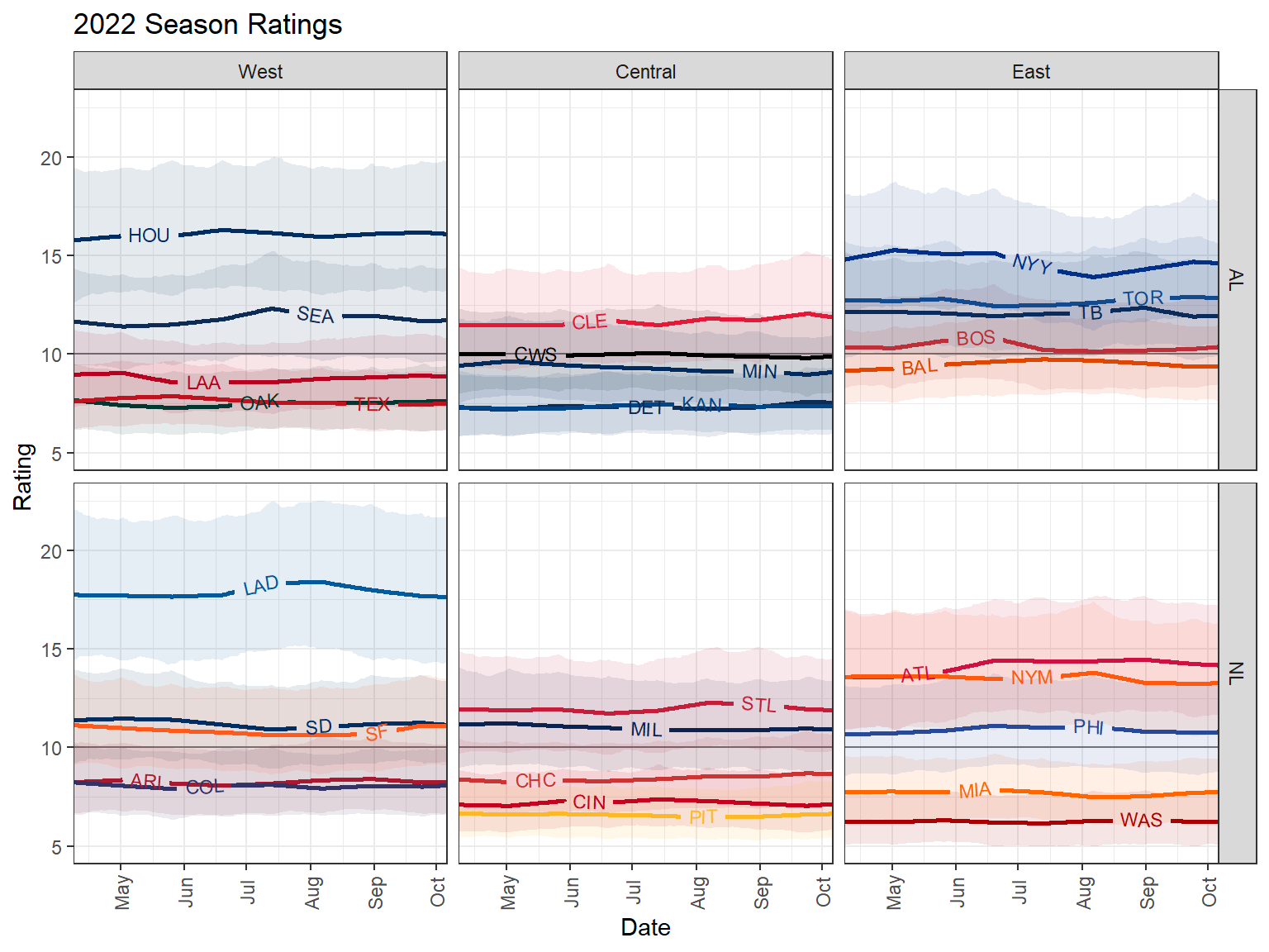
Let's look at the fitted ratings from the most recent season.
These have been scaled by 10, so that a value of 10 is average.
If a team with a rating of 12 plays a team with rating 8, the former team will have 12/8 or 3/2 odds of betting the latter (ignoring home-field advantage).
The graph below shows our best guess of team's ratings over the course of the season, along with 90% credible intervals.
[This is different from the graph we'd get if we used our model after every game and plotted our *contemporaneous* estimates of each team's ratings.]{.aside}
```{r ratings-prev}
d_ratings <- summary(draws[, , idx_rate], mean, ~ quantile2(., c(0.1, 0.9))) |>
  separate_wider_regex(variable, c("^ratings\\[", team = "\\d+", ",", day = "\\d+", "]")) |>
  transmute(
    team = factor(d_teams$team[as.integer(team)], d_teams$team),
    season = historical_season,
    day = as.integer(day),
    rate = 10 * exp(mean),
    q10 = 10 * exp(q10),
    q90 = 10 * exp(q90)
  )

d_ratings |>
  filter(day <= max(d$day[d$season == historical_season])) |>
  left_join(d_teams, by = "team") |>
  group_by(league, division, day) |>
  mutate(
    date = min(d$date[d$season == historical_season]) + day,
    i = row_number() / (n() + 1)
  ) |>
  ggplot(aes(date, rate, group = team)) +
  facet_grid(league ~ division) +
  geom_hline(yintercept = 10, color = "#777777") +
  geom_ribbon(aes(ymin = q10, ymax = q90, fill = primary), alpha = 0.1) +
  geom_textline(aes(color = primary, label = abbr, hjust = i), linewidth = 1.0, size = 3) +
  scale_color_identity() +
  scale_fill_identity() +
  scale_x_date(expand = c(0, 0)) +
  labs(x = "Date", y = "Rating", title = paste(historical_season, "Season Ratings")) +
  theme_bw() +
  theme(axis.text.x = element_text(angle = 90, vjust = 0.5))
```
Notice the relatively large amount of uncertainty.
Games are very evenly matched, and most pairs of teams don't play many games.
Still, we're able to distinguish teams with relatively high confidence:
- We are `r percent(Pr(rv_rate["HOU"] > rv_rate["SEA"]))` sure the Astros were better than the Mariners.
- We are `r percent(Pr(rv_rate["ATL"] > rv_rate["NYM"]))` sure the Braves were better than the Mets.
- We are `r percent(E(rdo(all(rv_rate["WAS"] < rv_rate[names(rv_rate) != "WAS"]))))` sure that the Nationals were worse than every other team.
We'll finish by summarizing the hyperparameters, so we can use them as priors for future seasons' ratings.
```{r fitdistr}
p <- ncol(model.matrix(form, d))
fits <- list(
  beta = do.call(rbind, map(seq_len(p), function(i) {
    MASS::fitdistr(as.numeric(draws[, , i]), "normal")$estimate
  })),
  rho = median(draws[, , "rho"]),
  sigma = MASS::fitdistr(as.numeric(draws[, , "sigma10"]), "gamma")$estimate * c(1, 10),
  alpha = median(draws[, , "alpha"]),
  tau_marg = sqrt((median(draws[, , "alpha"]) * median(draws[, , "sigma10"]) / 10)^2 +
    median(draws[, , "tau10"])^2 / 100), # adjust so we get right marginal variance for plug-in ests
  log_rate_final = d_ratings |>
    filter(day == max(d$day[d$season == historical_season])) |>
    transmute(team = team, season = season, rate = log(rate / 10))
)

if (!file.exists(path <- here("data/fit_hypers.rds"))) {
  write_rds(fits, path, compress = "xz")
}
```
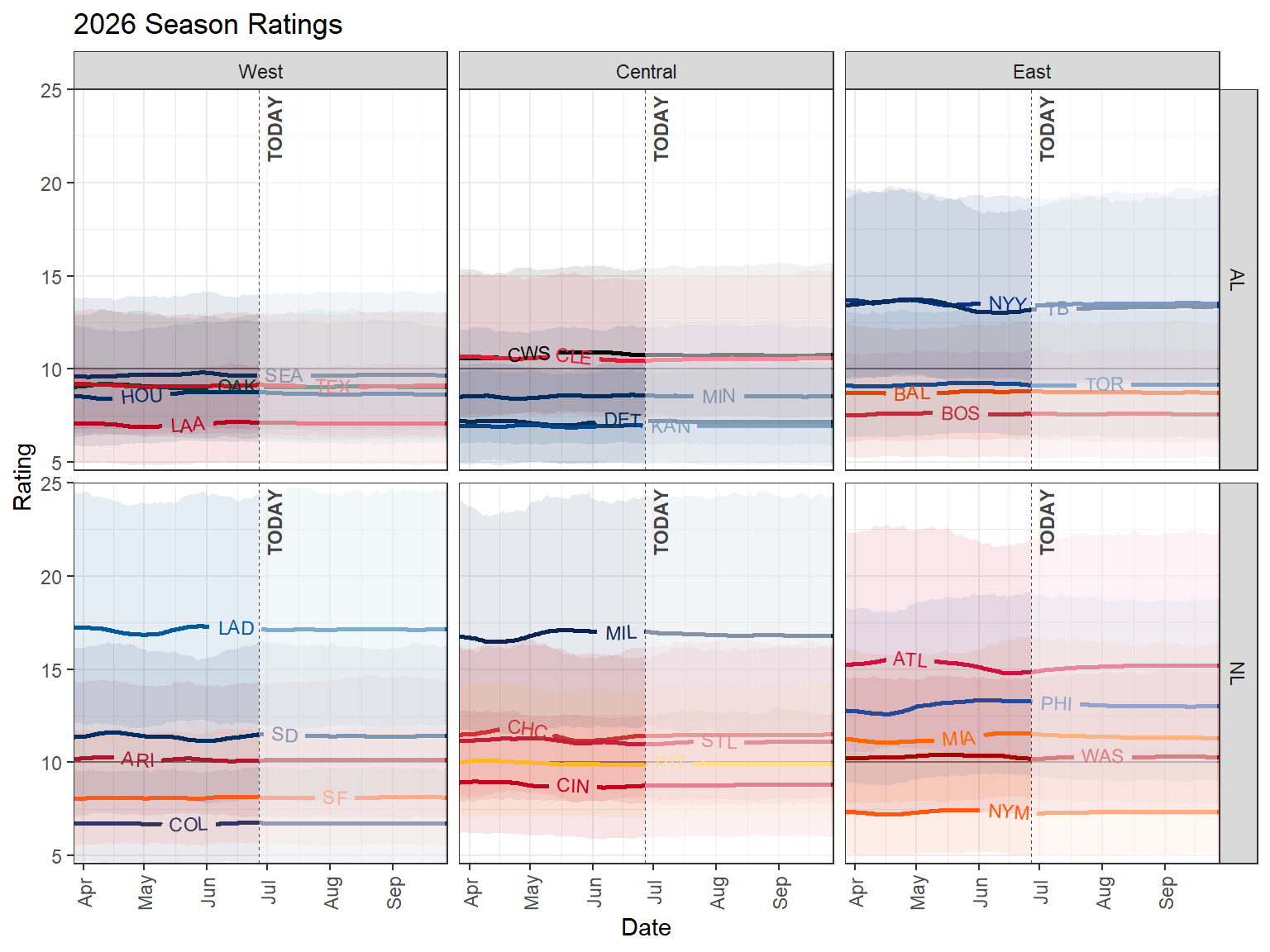
# Applying the model to the current season
We can then use these fitted parameters as priors in the same model fit to `r season` games.
We'll be a bit less confident in our prior on average ratings.
We'll also predict the results of future games using the generated quantities Stan block.
``` stan
generated quantities {
  array[N] int<lower=0,upper=1> res_pred;
  {
  vector[N] rate_diff;
  for (i in 1:N_pred) {
    rate_diff[i] = ratings[home_pred[i], home_pred[i]] -
        ratings[home_pred[i], home_pred[i]];
  }
  res_pred = bernoulli_logit_rng(rate_diff + X_pred*beta);
  }
}
```
```{r fit-new}
#| code-fold: true
#| code-summary: "Fit code"
d_current <- game_data_mlb(season)

prep_data_single <- function(d, fits, knot_space = 7) {
  d_compl <- filter(d, !is.na(result))
  d_pred <- filter(d, is.na(result), day >= max(d_compl$day))
  max_days <- max(d$day)
  m_spline <- splines::bs(seq_len(max_days),
    df = round(max_days / knot_space),
    degree = 1, intercept = TRUE
  )
  n_teams <- nlevels(d$home)
  X <- model.matrix(form, d_compl)

  list(
    `T` = n_teams,
    N = nrow(d_compl),
    N_pred = nrow(d_pred),
    D = max_days,
    K = ncol(m_spline),
    P = ncol(X),
    day = d_compl$day,
    home = as.integer(d_compl$home),
    away = as.integer(d_compl$away),
    result = as.integer(d_compl$result),
    X = X,
    day_pred = d_pred$day,
    home_pred = as.integer(d_pred$home),
    away_pred = as.integer(d_pred$away),
    X_pred = model.matrix(form, d_pred),
    knot_space = knot_space,
    splines = m_spline,
    prior_rate_loc = fits$log_rate_final$rate * fits$alpha,
    prior_rate_scale = 4 * rep(fits$tau_marg, n_teams),
    rho = fits$rho,
    prior_sigma_rate = fits$sigma["rate"],
    prior_sigma_shape = fits$sigma["shape"],
    prior_beta_scale = fits$beta[, "sd"],
    prior_beta_loc = fits$beta[, "mean"]
  )
}

hyperpars <- c("beta", "sigma10")
if (!file.exists(path <- here(str_glue("data/fit{season}.rds")))) {
  sm1 <- cmdstan_model(here("R/stan/ratings_single.stan"), stanc_options = list("O1"))

  fit_current <- sm1$sample(
    data = prep_data_single(d_current, fits, knot_space = 7),
    chains = 4, iter_warmup = 800, iter_sampling = 500, thin = 1,
    refresh = 100, adapt_delta = 0.85, step_size = 0.15
  )
  draws <- fit_current$draws(c(hyperpars, "ratings", "res_pred"))
  write_rds(draws, path, compress = "xz")
} else {
  draws <- read_rds(path)
}
```
We can make a similar ratings plot.
```{r ratings}
#| code-fold: true
#| code-summary: "Plot code"
idx <- which(str_starts(dimnames(draws)$variable, "rat"))
d_ratings <- summary(draws[, , idx], mean, ~ quantile2(., c(0.1, 0.9))) |>
  separate_wider_regex(variable, c("^ratings\\[", team = "\\d+", ",", day = "\\d+", "]")) |>
  transmute(
    team = factor(d_teams$team[as.integer(team)], d_teams$team),
    day = as.integer(day),
    rate = 10 * exp(mean),
    q10 = 10 * exp(q10),
    q90 = 10 * exp(q90)
  )

d_ratings |>
  filter(day <= max(d_current$day)) |>
  left_join(d_teams, by = "team") |>
  group_by(league, division, day) |>
  mutate(
    date = min(d_current$date) + day,
    i = row_number() / (n() + 2)
  ) |>
  ggplot(aes(date, rate, group = team)) +
  facet_grid(league ~ division) +
  geom_hline(yintercept = 10, color = "#777777") +
  geom_ribbon(aes(ymin = q10, ymax = q90, fill = primary), alpha = 0.1) +
  geom_textline(aes(color = primary, label = abbr, hjust = i), linewidth = 1.0, size = 3) +
  annotate("rect",
    xmin = today(), xmax = max(d_current$date), ymin = -Inf, ymax = Inf,
    fill = "white", alpha = 0.5
  ) +
  geom_vline(xintercept = today(), linewidth = 0.3, color = "#444444", lty = "dashed") +
  annotate("text",
    x = today(), y = 25, label = "TODAY", angle = 90,
    color = "#444444", fontface = "bold", hjust = 1.1, vjust = 1.5, size = 3
  ) +
  scale_color_identity() +
  scale_fill_identity() +
  coord_cartesian(expand = FALSE) +
  labs(x = "Date", y = "Rating", title = paste(season, "Season Ratings")) +
  theme_bw() +
  theme(axis.text.x = element_text(angle = 90, vjust = 0.5))
```
We can also use the model's future predictions to forecast the results at the end of the season.
```{r pred}
sum_wins <- function(x, fn = sum) {
  bind_rows(
    group_by(x, home) |>
      summarize(
        n = n(),
        wins = fn(result)
      ) |>
      rename(team = home),
    group_by(x, away) |>
      summarize(
        n = n(),
        wins = n - fn(result)
      ) |>
      rename(team = away)
  ) |>
    group_by(team) |>
    summarize(
      wins = fn(wins),
      n = sum(n)
    )
}

d_won <- filter(d_current, !is.na(result)) |>
  sum_wins()
d_pred <- filter(d_current, is.na(result), day >= max(d_current$day[!is.na(d_current$result)])) |>
  mutate(result = as_draws_rvars(draws, .nchains = fit_current$num_chains())$res_pred) |>
  sum_wins(fn = rvar_sum) |>
  left_join(d_won, by = "team", suffix = c("_pred", "")) |>
  transmute(
    team = team,
    wins = wins + wins_pred,
    n = n + n_pred
  )

in_playoffs <- function(x, div) {
  rk <- rank(x, ties.method = "random")
  leaders <- which(rk %in% tapply(rk, div, max))
  out <- logical(length(x))
  out[leaders] <- TRUE
  out[-leaders] <- rank(rk[-leaders]) > 9
  out
}

d_rate <- d_ratings |>
  filter(day == today() - min(d_current$date) + 1L) |>
  select(team, rate)

d_pred |>
  mutate(wins = wins * 162 / n) |>
  left_join(d_teams, by = "team") |>
  group_by(league, division) |>
  mutate(win_division = Pr(rdo(rank(wins, ties.method = "random")) > 4)) |>
  group_by(league) |>
  mutate(make_playoffs = Pr(rdo(in_playoffs(wins, division)))) |>
  ungroup() |>
  arrange(league, division, desc(E(wins))) |>
  group_by(league, division) |>
  left_join(d_rate, by = "team") |>
  select(
    team = mascot, league, division, Rating = rate, Wins = wins,
    `Win division` = win_division, `Make playoffs` = make_playoffs
  ) |>
  gt(rowname_col = "team") |>
  tab_header(title = paste(season, "Season Predictions")) |>
  tab_stubhead("Team") |>
  fmt_number(decimals = 1) |>
  fmt_percent(columns = c("Win division", "Make playoffs"), decimals = 1) |>
  data_color(
    columns = c("Win division", "Make playoffs"),
    fn = col_numeric(wacolors::wacolors$lopez[c(8, 15)], 0:1)
  ) |>
  data_color(columns = "Rating", fn = col_numeric(wacolors::wacolors$lopez, c(1, 23)))
```