---
title: Building a Bayesian Position Player WAR Model
date: last-modified
format:
html:
code-fold: show
code-tools: true
toc: true
code-annotations: below
fig-width: 7
fig-height: 5
fig-format: retina
fig-responsive: true
embed-resources: false
params:
season: 2026
execute:
warning: false
---
```{r setup}
#| code-fold: true
#| code-summary: "Setup code"
suppressPackageStartupMessages({
  library(cmdstanr)
  library(posterior)
  library(scales)
  library(ggrepel)
  library(gt)
  library(here)
  library(tidyverse)

  devtools::load_all()
})

season <- params$season
rpw <- fg_woba_weights(season)$rpw

pos_adj_per_600pa <- c(
  C = 12.5, SS = 7.5,
  `2B` = 2.5, `3B` = 2.5, CF = 2.5,
  LF = -7.5, RF = -7.5,
  `1B` = -12.5, DH = -17.5,
  OF = -7.5
)
```
# The Goal
Position player WAR estimates how many wins a player contributed above a replacement-level baseline.
Replacement level represents the freely-available minor league call-up a team could use instead.
Like our [Pitcher WAR model](pitcher_war_expl.qmd), this model is fully Bayesian.
The key advantage is uncertainty quantification: every player gets a full posterior distribution over WAR, with credible intervals that widen for players with few plate appearances.
Position player WAR has five components:
$$
\text{WAR} = \frac{\text{Batting} + \text{Fielding} + \text{Baserunning} + \text{Positional Adjustment} + \text{Replacement Runs}}{\text{Runs per Win}}
$$
| Component | What it measures | How we estimate it |
|-----------|-----------------|-------------------|
| Batting | Offensive value above/below average | Bayesian wOBA model (per-game logs) |
| Fielding | Defensive value above/below average | Bayesian shrinkage of DRS (framing runs for catchers) |
| Baserunning | Value on the bases beyond batting | Seasonal UBR + wSB (observed) |
| Positional Adj. | Difficulty of playing the position | Fixed constants (FanGraphs standard) |
| Replacement Runs | Credit for being available at all | ~20 runs per 600 PA below average |
# The Data
## Batting: per-game logs
The unit of observation for batting is a single **game appearance**.
Each game contributes six count outcomes to the likelihood:
| Symbol | Meaning |
|--------|---------|
| $y_{HR}$ | Home runs |
| $y_{3B}$ | Triples |
| $y_{2B}$ | Doubles |
| $y_{1B}$ | Singles (direct `1B` column) |
| $y_{BB}$ | Unintentional walks ($BB - IBB$) |
| $y_{HBP}$ | Hit by pitch |
Each game also records plate appearances (PA) as the exposure, the batter identity, the game date, and park factors for HR, 3B, 2B, and 1B.
```{r data-glimpse}
#| code-fold: true
#| code-summary: "Load and preview batting data"
d_logs <- read_rds(here(str_glue('data/batter_logs_{season}.rds')))
d_logs |>
  slice_sample(n = 8) |>
  select(name, team, date, pa, n_hr, n_3b, n_2b, n_1b, n_bb, n_hbp) |>
  arrange(date) |>
  gt() |>
  tab_header(title = 'Sample game-log rows') |>
  fmt_date(columns = date, date_style = 'yMMMd')
```
The data covers all batters with at least 1 PA in the season, roughly 700 players.
The first season fetch makes around 650 API calls to FanGraphs (one per batter) and is cached as a compressed `.rds` file.
## wOBA linear weights
Not all hits are equal.
A home run is worth more than a single.
**wOBA** (weighted on-base average) assigns run-value weights to each event:
$$
\text{wOBA} = \frac{w_{BB} \cdot BB + w_{HBP} \cdot HBP + w_{1B} \cdot 1B + w_{2B} \cdot 2B + w_{3B} \cdot 3B + w_{HR} \cdot HR}{\text{PA} - \text{IBB}}
$$
The weights come from linear-weight run expectancy calculations and are re-estimated each season by FanGraphs.
```{r woba-weights-table}
#| code-fold: true
#| code-summary: "Fetch and display wOBA weights"
woba_wts <- fg_woba_weights(season)
tibble(
  Event = c('Walk (unint.)', 'Hit by Pitch', 'Single', 'Double', 'Triple', 'Home Run'),
  Symbol = c('BB', 'HBP', '1B', '2B', '3B', 'HR'),
  Weight = c(
    woba_wts$w_bb, woba_wts$w_hbp, woba_wts$w_1b,
    woba_wts$w_2b, woba_wts$w_3b, woba_wts$w_hr
  )
) |>
  gt() |>
  tab_header(
    title = str_glue('{season} wOBA linear weights'),
    subtitle = 'Source: FanGraphs guts page'
  ) |>
  fmt_number(columns = Weight, decimals = 3) |>
  tab_footnote(
    footnote = str_glue(
      'wOBA scale = {round(woba_wts$woba_scale, 3)}; ',
      'league wOBA = {round(woba_wts$lg_woba, 3)}; ',
      'runs per win = {round(woba_wts$rpw, 2)}'
    )
  )
```
## Fielding: seasonal DRS
**DRS** (Defensive Runs Saved, Baseball Info Solutions) measures how many runs above or below average a fielder saved.
DRS is only available as a seasonal total (not per-game), so the fielding sub-model uses a different approach than the batting model.
We use DRS rather than UZR or FRP because it has a consistent methodology and column name from ~2003 to present — essential for future cross-year random-walk smoothing where UZR (discontinued after 2024) and FRP (introduced in 2025) cannot form a consistent series.
For catchers, we use **framing runs** (`CFraming`) from the FanGraphs fielding leaderboard.
This measures the run value of converting borderline pitches into called strikes.
## Baserunning: seasonal UBR + wSB
**UBR** (Ultimate Base Running) measures extra-base-advancement value on non-stolen-base plays.
**wSB** (weighted stolen base runs) captures stolen base and caught stealing.
We use FanGraphs seasonal values directly as point estimates.
# The Batting Model
The batting model is the statistical core of position player WAR.
It extends the [pitcher FIP model](pitcher_war_expl.qmd) from three components to six, using the same two-level hierarchy.
## League baseline
For each of the six event types $c \in \{HR, 3B, 2B, 1B, BB, HBP\}$, the league-average rate on day $d$ follows a **B-spline** on the logit scale:
$$
\text{logit}\bigl(\lambda^{(c)}_d\bigr) = \sum_{k=1}^{K} B_{dk} \cdot \theta^{(c)}_k
$$
where $B_{dk}$ is the spline basis matrix (knots every 14 days) and $\theta^{(c)}_k$ are the knot values.
A **random-walk prior** anchors the first knot near the observed league rate and allows slow drift:
$$
\theta^{(c)}_1 \sim \mathcal{N}(\text{logit}(\hat\lambda^{(c)}),\; 0.3), \quad
\theta^{(c)}_k \sim \mathcal{N}(\theta^{(c)}_{k-1},\; 0.1) \quad k \geq 2
$$
This captures real seasonal trends (e.g., a home run spike in warm weather) without overfitting to week-to-week noise.
## Batter offsets
Each batter $p$ has a scalar offset for each event type, estimated with **partial pooling** (non-centred parametrisation):
$$
\alpha^{(c)}_p = \sigma_c \cdot z^{(c)}_p, \quad z^{(c)}_p \sim \mathcal{N}(0,1), \quad \sigma_c \sim \mathcal{N}^+(0, 0.25)
$$
The shared scale $\sigma_c$ controls how much batter-to-batter variation the model finds for that component.
When $\sigma_c$ is small, all batters look alike and everyone is shrunk toward the league mean.
When $\sigma_c$ is large, individual batters diverge substantially.
## Likelihood
The expected count for event type $c$ in game $g$ is:
$$
\mu^{(c)}_g = \text{PA}_g \cdot \text{logit}^{-1}\!\Bigl(\lambda^{(c)}_{d_g} + \alpha^{(c)}_{p_g}\Bigr) \cdot \text{PF}^{(c)}_g
$$
where $\text{PF}^{(c)}_g = \exp(\log(\text{pf}^{(c)}_g / 100))$ is the park factor for component $c$ in game $g$.
HR, 3B, 2B, and 1B are park-adjusted using FanGraphs component park factors.
BB and HBP are not park-adjusted: walk rate is primarily a pitcher-batter interaction, and HBP has no reliable park factor.
Each count follows a **Negative Binomial** distribution to accommodate overdispersion beyond Poisson.
Real batters have slumps and hot streaks that inflate variance beyond what Poisson predicts:
$$
y^{(c)}_g \sim \text{NegBin}\bigl(\mu^{(c)}_g,\; \phi_c\bigr), \quad \phi_c \sim \text{Gamma}(3, 0.1)
$$
## Full Stan model
```{stan}
#| label: batting-stan
#| echo: true
#| eval: false
#| output.var: batting_model
#| file: R/stan/batting_war.stan
```
# From wOBA to Batting WAR
After sampling, we compute per-batter wOBA and WAR in R from the posterior draws, following the same post-processing pattern as pitcher WAR.
## wOBA per PA
In the **generated quantities** block, each posterior draw gives true per-PA rates $r^{(c)}_p$ for all six event types:
$$
r^{(c)}_p = \text{logit}^{-1}\!\bigl(\bar\lambda^{(c)} + \alpha^{(c)}_p\bigr)
$$
where $\bar\lambda^{(c)}$ is the season-average league logit rate.
Then:
$$
\text{wOBA}_p = w_{HR}\,r^{HR}_p + w_{3B}\,r^{3B}_p + w_{2B}\,r^{2B}_p + w_{1B}\,r^{1B}_p + w_{BB}\,r^{BB}_p + w_{HBP}\,r^{HBP}_p
$$
The FanGraphs weights $w_c$ are already on the wOBA scale (each equals the raw linear weight $\times$ wOBA scale), so the sum gives wOBA directly.
## wRAA per PA
Batting runs above average per plate appearance:
$$
\text{wRAA/PA}_p = \frac{\text{wOBA}_p - \overline{\text{wOBA}}_\text{lg}}{\text{wOBA scale}}
$$
## Batting WAR
```{r batting-war-post}
#| code-fold: true
#| code-summary: "Batting WAR post-processing"
draws_bat <- read_rds(here(str_glue('data/fit_batting_{season}.rds')))
d_logs <- read_rds(here(str_glue('data/batter_logs_{season}.rds')))
woba_wts <- fg_woba_weights(season)
batting_stan <- prep_batting_stan(
d_logs,
tryCatch(fg_batting_park(season), error = \(e) NULL),
woba_wts
)
d_pa <- d_logs |>
group_by(player_id, name) |>
summarise(pa = sum(pa), team = last(team), .groups = 'drop')
wraa_mat <- as_draws_matrix( # <1>
draws_bat[, , str_starts(variables(draws_bat), 'wraa_per_pa')]
)
pa_vec <- d_pa$pa[match(batting_stan$batter_levels, d_pa$player_id)] # <2>
batting_runs_mat <- sweep(wraa_mat, 2, pa_vec, '*') # <3>
repl_mat <- outer(rep(1L, nrow(batting_runs_mat)), 20 * pa_vec / 600) # <4>
batting_war_mat <- (batting_runs_mat + repl_mat) / woba_wts$rpw # <5>
```
1. Pull the `wraa_per_pa` draws: a matrix of [draws × batters].
2. Align PA totals to the Stan batter-index ordering.
3. Multiply each batter's wRAA/PA by their actual PA to get season wRAA.
4. Add replacement-level credit: ~20 runs below average per 600 PA.
5. Divide by runs-per-win to convert to WAR scale.
The **replacement level** of 20 runs per 600 PA reflects that a bench player or call-up typically bats around 20 runs below the league average.
Every PA from an above-replacement player is that much more valuable than what a team could freely get.
# Defense: DRS and Bayesian Shrinkage
## The DRS reliability problem
DRS is noisy at the single-season level.
Its year-to-year correlation for a single season is roughly $r \approx 0.2$–$0.3$, somewhat lower than UZR.
A player who appears to save 15 runs in one year might truly be a 5-run saver, or even a −2-run saver.
The Bayesian solution is to treat each season's DRS as a **noisy measurement** of the player's true defensive talent, with noise that decreases as playing time increases.
## The measurement error model
For non-catcher fielder $p$ at position $j$, the model uses a **rate parametrisation**: the prior is placed on the player's true defensive rate per full season, and the actual run contribution scales with innings played.
$$
\tau_p \sim \mathcal{N}(0,\; \sigma^{(j)}_\text{talent})
$$
$$
\text{DRS}_p \sim \mathcal{N}\!\Bigl(\tau_p \cdot \frac{\text{inn}_p}{1350},\; \frac{\sigma^{(j)}_\text{meas}}{\sqrt{\text{inn}_p / 1350}}\Bigr)
$$
where $\tau_p$ is the true rate (runs per full season), $\sigma^{(j)}_\text{talent}$ is the SD of talent at position $j$, and $\sigma^{(j)}_\text{meas}$ is the measurement noise at full exposure.
A player with 200 innings is expected to contribute ~15% of a full season's worth of runs; the model does not need to learn this from data — it is built into the mean of the likelihood.
### Why sigma_meas cannot be estimated from a single season
There is a structural identification problem: the model has one latent parameter $z_p$ per player.
The sampler can always explain every player's observed DRS by setting $z_p = \text{obs\_drs}_p / (\sigma_\text{talent} \cdot v_p)$ — i.e., treating observed DRS as exact truth — and then driving $\sigma_\text{meas} \to 0$.
This degeneracy holds regardless of parametrisation or prior shape: with ~500 players all pulling $\sigma_\text{meas}$ toward 0, even a strong lognormal prior is overwhelmed.
Resolving $\sigma_\text{meas}$ from $\sigma_\text{talent}$ requires *repeated measurements of the same players* — either across seasons or within a season via split samples.
That is the natural setting for a multi-season random-walk model, deferred to a future version.
### Fixing sigma_meas via known reliability (empirical Bayes)
Since $\sigma_\text{meas}$ cannot be estimated from one season, we fix its *ratio* to $\sigma_\text{talent}$ using the known DRS year-to-year reliability $r$:
$$
r = \frac{\sigma^2_\text{talent}}{\sigma^2_\text{talent} + \sigma^2_\text{meas}}
\quad\Longrightarrow\quad
\frac{\sigma_\text{meas}}{\sigma_\text{talent}} = \sqrt{\frac{1-r}{r}} =: \rho
$$
With $r_\text{DRS} \approx 0.40$, $\rho \approx 1.22$.
Only $\sigma^{(j)}_\text{talent}$ is estimated from the current season's cross-sectional data; $\sigma^{(j)}_\text{meas} = \rho \cdot \sigma^{(j)}_\text{talent}$ is derived.
This is standard **empirical Bayes**: substituting external knowledge for a parameter the data cannot pin down.
The implied shrinkage for a player with $v = \text{inn}/1350$ is:
$$
\mathbb{E}[\tau_p \mid \text{DRS}_p] = \text{DRS}_p \cdot \frac{r}{r + (1-r)/v}
$$
| Innings | $v$ | Shrinkage factor | Interpretation |
|---------|-----|-----------------|----------------|
| 1350 (full) | 1.00 | $r = 0.40$ | Full-season player: 40% of observed DRS is credited |
| 675 (half) | 0.50 | 0.25 | Half-season: 25% credited |
| 200 | 0.15 | 0.09 | Part-season: 9% credited, strongly pooled toward 0 |
A player with 1350 innings gets noise $\sigma^{(j)}_\text{meas}$; a player with 338 innings gets noise $2 \times \sigma^{(j)}_\text{meas}$, reflecting four times less information.
## Shrinkage in action
```{r fielding-shrinkage}
#| code-fold: true
#| code-summary: "Fielding shrinkage plot"
d_field <- read_rds(here(str_glue('data/fielding_{season}.rds')))
d_framing <- read_rds(here(str_glue('data/framing_{season}.rds')))
draws_fld <- read_rds(here(str_glue('data/fit_fielding_{season}.rds')))
fld_stan <- prep_fielding_stan(d_field, d_framing)
drs_post_med <- apply(
as_draws_matrix(draws_fld[, , str_starts(variables(draws_fld), 'true_drs')]),
2, median
)
tibble(
player_id = fld_stan$fielder_levels,
drs_post = drs_post_med
) |>
left_join(fld_stan$d_field_agg, by = 'player_id') |>
ggplot(aes(drs, drs_post)) +
geom_abline(slope = 1, intercept = 0, color = '#888888', linewidth = 0.5) +
geom_hline(yintercept = 0, color = '#e6550d', linewidth = 0.4, lty = 'dotted') +
geom_point(aes(size = inn), alpha = 0.4, color = '#31a354') +
geom_text_repel(
data = ~ filter(.x, inn < 400 | abs(drs - drs_post) > 8),
aes(label = player_id),
size = 2.6,
max.overlaps = 12,
seed = 42
) +
scale_size_continuous(range = c(0.5, 4), name = 'Innings') +
labs(
x = 'Observed DRS (runs)',
y = 'Posterior median true DRS (runs)',
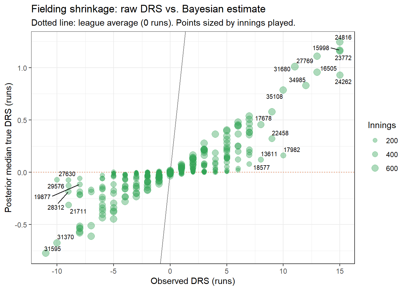
title = 'Fielding shrinkage: raw DRS vs. Bayesian estimate',
subtitle = 'Dotted line: league average (0 runs). Points sized by innings played.'
) +
theme_bw(base_size = 11)
```
Players with few innings are pulled strongly toward zero.
Players with a full season of data stay close to their observed DRS.
The model learns $\sigma^{(j)}_\text{meas}$ and $\sigma^{(j)}_\text{talent}$ from the entire league, so the shrinkage is calibrated rather than arbitrary.
# Catcher Framing
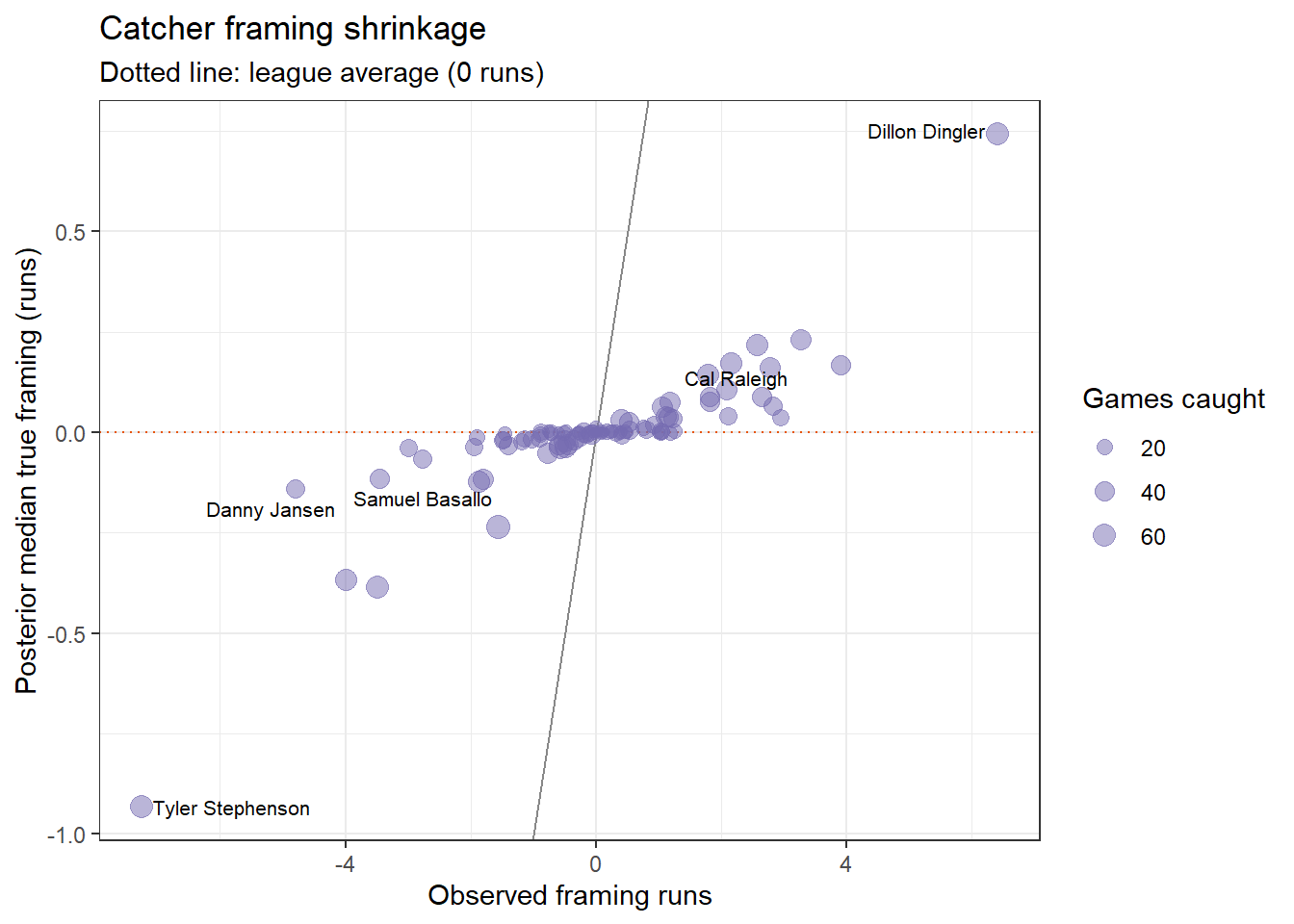
Catchers have a unique defensive skill: influencing umpires to call borderline pitches as strikes.
**Framing runs** (`CFraming` from FanGraphs) measure this directly as a run value.
Elite framers can save 15–20 runs per season, comparable to outstanding infield defense.
The framing model mirrors the DRS model: observed framing runs equal true talent plus noise, shrinking toward zero for catchers with few games caught.
```{r framing-shrinkage}
#| code-fold: true
#| code-summary: "Catcher framing shrinkage plot"
if (length(fld_stan$catcher_levels) > 0) {
  frame_post_med <- apply(
    as_draws_matrix(draws_fld[, , str_starts(variables(draws_fld), 'true_framing')]),
    2, median
  )

  tibble(
    player_id = fld_stan$catcher_levels,
    framing_post = frame_post_med
  ) |>
    left_join(d_framing, by = 'player_id') |>
    ggplot(aes(framing_runs, framing_post)) +
    geom_abline(slope = 1, intercept = 0, color = '#888888', linewidth = 0.5) +
    geom_hline(yintercept = 0, color = '#e6550d', linewidth = 0.4, lty = 'dotted') +
    geom_point(aes(size = games_caught), alpha = 0.5, color = '#756bb1') +
    geom_text_repel(
      data = ~ filter(.x, games_caught < 40 | abs(framing_runs - framing_post) > 5),
      aes(label = name),
      size = 2.8,
      max.overlaps = 12,
      seed = 42
    ) +
    scale_size_continuous(range = c(1, 4), name = 'Games caught') +
    labs(
      x = 'Observed framing runs',
      y = 'Posterior median true framing (runs)',
      title = 'Catcher framing shrinkage',
      subtitle = 'Dotted line: league average (0 runs)'
    ) +
    theme_bw(base_size = 11)
} else {
  cat('No catcher framing data available for this season.')
}
```
# Baserunning
Total baserunning value is the sum of two components:
| Component | Measures |
|-----------|----------|
| **UBR** | Extra bases taken on hits, outs on the bases, other advancement decisions |
| **wSB** | Value of stolen base attempts: $\text{wSB} = 0.2 \times SB - 0.4 \times CS$ (approximately) |
We use the FanGraphs seasonal values directly as point estimates.
These are already computed using run-expectancy linear weights, so they're on the same scale as batting runs and DRS.
Baserunning values are smaller than batting or fielding, typically ranging from −5 to +5 runs, and their year-to-year reliability is moderate.
An additional layer of Bayesian shrinkage is possible but low-priority for this model version.
# Positional Adjustments
Not all positions require equal skill.
A shortstop who bats identically to a first baseman is more valuable, because the shortstop provides defense the team could not easily replace.
We apply a **fixed positional adjustment** per 600 PA, reflecting the offensive opportunity cost of playing each position:
```{r pos-adj-table}
#| code-fold: true
#| code-summary: "Positional adjustment table"
tibble(
  Position = c(
    'Catcher', 'Shortstop', 'Second Base', 'Third Base', 'Center Field',
    'Left/Right Field', 'First Base', 'Designated Hitter'
  ),
  Abbrev = c('C', 'SS', '2B', '3B', 'CF', 'LF/RF', '1B', 'DH'),
  `Runs/600PA` = c(12.5, 7.5, 2.5, 2.5, 2.5, -7.5, -12.5, -17.5)
) |>
  gt() |>
  tab_header(
    title = 'Positional adjustments (FanGraphs standard)',
    subtitle = 'Runs above average per 600 plate appearances'
  ) |>
  fmt_number(columns = `Runs/600PA`, decimals = 1) |>
  data_color(
    columns = `Runs/600PA`,
    fn = col_numeric(c('#d73027', '#fee090', '#74add1'), domain = c(-18, 13))
  )
```
These constants are well-established and would require multi-decade data to estimate reliably from scratch.
The positional adjustment is scaled by actual PA / 600, so a catcher who played 400 PA receives $12.5 \times (400/600) \approx 8.3$ runs of positional credit.
# Putting It Together
## WAR aggregation
All components are combined in R from posterior draws:
```{r war-agg-demo}
#| code-fold: true
#| code-summary: "WAR aggregation (abridged)"
# This is the same code as in position_war.qmd post-process chunk.
# Shown here for illustration with a minimal example.

# 1. Batting WAR from posterior wraa_per_pa draws
# war_mat[i, p] = posterior draw i, batter p
batting_war_mat_demo <- (sweep(wraa_mat, 2, pa_vec, '*') + # wRAA × PA
  outer(rep(1, nrow(wraa_mat)), 20 * pa_vec / 600)) / # + replacement
  woba_wts$rpw # ÷ RPW

# 2. Point estimates for fielding, baserunning, positional
# (computed similarly from fielding draws and seasonal data)

# 3. Total WAR combines all components; CI spans batting + fielding uncertainty
d_war <- tibble(
  player_id = batting_stan$batter_levels,
  batting_war_med = apply(batting_war_mat_demo, 2, median),
  batting_war_lo = apply(batting_war_mat_demo, 2, quantile, 0.10),
  batting_war_hi = apply(batting_war_mat_demo, 2, quantile, 0.90)
) |>
  left_join(d_pa, by = 'player_id') |>
  arrange(desc(batting_war_med))

cat('Top 5 by batting WAR contribution:\n')
d_war |>
  slice_head(n = 5) |>
  select(name, pa, batting_war_med, batting_war_lo, batting_war_hi) |>
  gt() |>
  fmt_number(columns = c(batting_war_med, batting_war_lo, batting_war_hi), decimals = 1) |>
  cols_label(batting_war_med = 'Bat WAR', batting_war_lo = '10th', batting_war_hi = '90th')
```
# Comparison with FanGraphs fWAR
Our Bayesian WAR and FanGraphs fWAR answer the same question but with different methods.
Key differences:
| Aspect | This model | FanGraphs fWAR |
|--------|-----------|---------------|
| Batting estimation | Hierarchical Bayesian + partial pooling | Direct wOBA calculation |
| Defense estimation | Gaussian shrinkage model on DRS (absolute-value parametrisation) | Regressed UZR/FRP (3-year average) |
| Uncertainty | Full posterior distributions | Point estimates |
| Low-PA players | Heavily shrunk toward mean | Minimum PA threshold applied |
| Park adjustment | HR, 1B, 2B, 3B component factors on log scale | Separate multi-factor park adjustment |
```{r fwar-comparison}
#| code-fold: true
#| code-summary: "Correlation with FanGraphs fWAR"
# Retrieve FanGraphs fWAR from the batter leaders response
# (the WAR column is available in the same API call as batter IDs)
fg_war <- tryCatch(
fg_batter_ids(season) |>
transmute(player_id = playerid, fg_war = WAR),
error = function(e) NULL
)
if (!is.null(fg_war)) {
d_compare <- d_war |>
left_join(fg_war, by = 'player_id') |>
filter(!is.na(fg_war), pa >= 100)
r_val <- round(cor(d_compare$batting_war_med, d_compare$fg_war, use = 'complete.obs'), 3)
d_compare |>
ggplot(aes(fg_war, batting_war_med)) +
geom_abline(slope = 1, intercept = 0, color = '#888888', linewidth = 0.5, lty = 'dashed') +
geom_point(aes(size = pa), alpha = 0.4, color = '#3182bd') +
geom_smooth(method = 'lm', se = FALSE, color = '#e6550d', linewidth = 0.8) +
geom_text_repel(
data = ~ slice_max(.x, abs(fg_war - batting_war_med), n = 15),
aes(label = name),
size = 2.6,
seed = 42
) +
scale_size_continuous(range = c(0.5, 4), name = 'PA') +
labs(
x = 'FanGraphs fWAR',
y = 'Bayesian Batting WAR (posterior median)',
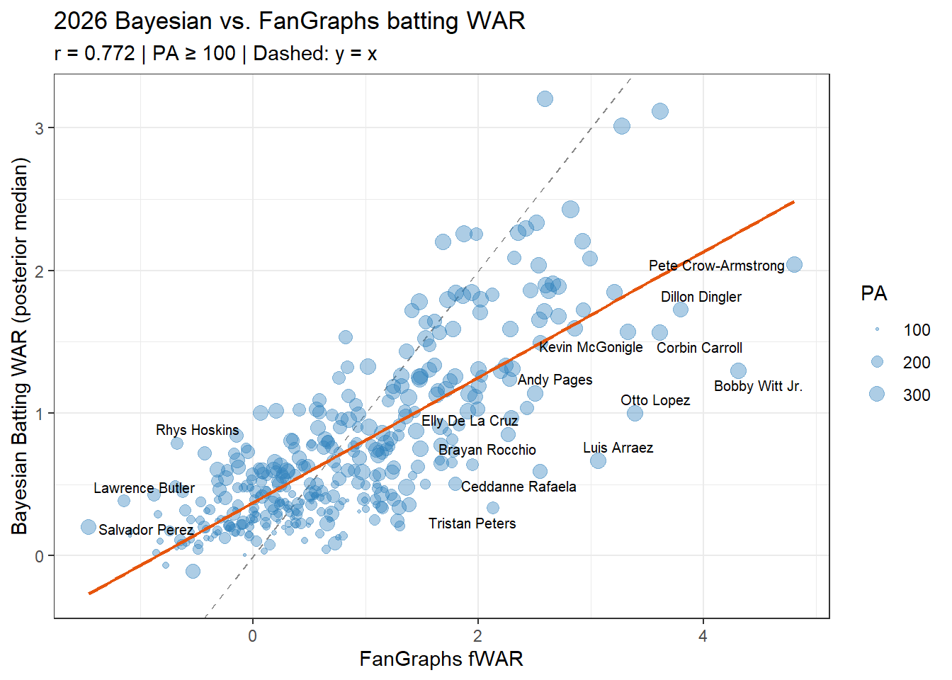
title = str_glue('{season} Bayesian vs. FanGraphs batting WAR'),
subtitle = str_glue('r = {r_val} | PA \u2265 100 | Dashed: y = x')
) +
theme_bw(base_size = 11)
} else {
cat('FanGraphs fWAR data not available for comparison.')
}
```
The Bayesian estimates and fWAR should correlate strongly (target: $r > 0.85$).
Large outliers are typically low-PA players where Bayesian shrinkage pulls the estimate toward zero, while fWAR uses the raw observed value.
# Validation
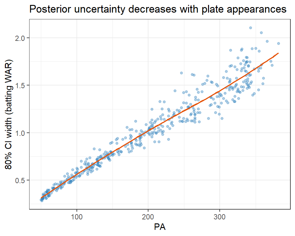
## Posterior uncertainty decreases with PA
A well-functioning model should have narrower credible intervals for players with more data.
```{r validation-ci}
#| fig-height: 4
#| fig-width: 5
d_war |>
  filter(pa >= 50) |>
  mutate(ci_width = batting_war_hi - batting_war_lo) |>
  ggplot(aes(pa, ci_width)) +
  geom_point(alpha = 0.4, size = 1.2, color = '#3182bd') +
  geom_smooth(method = 'loess', se = FALSE, color = '#e6550d', linewidth = 0.8) +
  labs(
    x = 'PA',
    y = '80% CI width (batting WAR)',
    title = 'Posterior uncertainty decreases with plate appearances'
  ) +
  theme_bw(base_size = 11)
```
## Total WAR sanity check
Position players account for roughly 55–60% of total WAR.
With pitchers expected to generate 150–200 WAR per full season, position players should generate around 500–650 WAR.
```{r validation-totals}
full_war <- read_rds(here(str_glue('data/fit_batting_{season}.rds')))
d_all_pa <- read_rds(here(str_glue('data/batter_logs_{season}.rds'))) |>
  group_by(player_id) |>
  summarise(pa = sum(pa), .groups = 'drop')

season_scale <- min(1, (as.integer(
  max(read_rds(here(str_glue('data/batter_logs_{season}.rds')))$date) -
    min(read_rds(here(str_glue('data/batter_logs_{season}.rds')))$date)
) + 1) / 186)

cat(str_glue(
  'Season scale factor: {round(season_scale, 3)}\n',
  'Expected batting + other WAR: ~{round(500 * season_scale)}\u2013{round(650 * season_scale)}\n'
))
```
## wOBA league average check
The league wOBA computed from game logs should match the FanGraphs published value within 0.002.
A larger discrepancy indicates a data pipeline issue.
```{r validation-woba}
woba_wts <- fg_woba_weights(season)
d_logs <- read_rds(here(str_glue('data/batter_logs_{season}.rds')))

lg_totals <- d_logs |>
  summarise(across(c(pa, n_hr, n_3b, n_2b, n_1b, n_bb, n_hbp), sum))

computed_woba <- with(
  lg_totals,
  (woba_wts$w_hr * n_hr + woba_wts$w_3b * n_3b + woba_wts$w_2b * n_2b +
    woba_wts$w_1b * n_1b + woba_wts$w_bb * n_bb + woba_wts$w_hbp * n_hbp) / pa
)

diff <- abs(computed_woba - woba_wts$lg_woba)
flag <- if (diff > 0.002) '\u26a0 exceeds tolerance' else '\u2713 within tolerance'
cat(str_glue(
  'Computed lg wOBA: {round(computed_woba, 4)}\n',
  'FanGraphs lg wOBA: {round(woba_wts$lg_woba, 4)}\n',
  'Difference: {round(diff, 4)} {flag}\n'
))
```