Setup code
suppressPackageStartupMessages({
  library(cmdstanr)
  library(posterior)
  library(scales)
  library(ggrepel)
  library(gt)
  library(here)
  library(tidyverse)

  devtools::load_all()
})suppressPackageStartupMessages({
library(cmdstanr)
library(posterior)
library(scales)
library(ggrepel)
library(gt)
library(here)
library(tidyverse)
devtools::load_all()
})Pitcher WAR estimates how many wins a pitcher contributed above a replacement-level baseline. We use FIP (Fielding Independent Pitching) as the underlying performance metric. K, BB, and HR rates are the outcomes most directly under a pitcher’s control, and the least contaminated by defense and sequencing.
The model has two levels. At the league level, a time-varying spline tracks how K/BB/HR rates drift across a season. At the pitcher level, each pitcher has a scalar offset relative to that baseline, estimated with partial pooling. Pitchers with many innings earn precise, data-driven estimates. Pitchers with few starts are pulled toward the league mean. The result is a full posterior distribution over WAR for each pitcher, with credible intervals that reflect how much the data supports the estimate.
The model is fit separately for starters and relievers. Starters and relievers have different replacement levels and — for relievers — leverage-weighted innings.
The unit of observation is a single start. Each start contributes three count outcomes to the likelihood:
| Symbol | Meaning |
|---|---|
| \(y_K\) | Strikeouts + IFFB (infield fly balls are automatic outs) |
| \(y_{BB}\) | BB + HBP \(-\) IBB (free baserunners, intentional walks excluded) |
| \(y_{HR}\) | Home runs |
Each start also records batters faced (BFP) as the exposure, the pitcher identity, the game date, and the park HR factor.
Per-start game logs come from FanGraphs via baseballr, about 150 API calls per season. Results are cached as .rds on first run.
season <- params$season
d_logs <- read_rds(here(str_glue('data/pitcher_logs_{season}.rds')))
stan_dat <- prep_pitcher_stan(d_logs, NULL, knot_space = 14)
draws <- read_rds(here(str_glue('data/fit_pitcher_{season}.rds')))
Here is a random sample of starts:
d_logs |>
  slice_sample(n = 8) |>
  select(name, team, date, bfp, ip, k_aut, bb_free, hr) |>
  arrange(date) |>
  knitr::kable(
    col.names = c(
      'Pitcher',
      'Team',
      'Date',
      'BFP',
      'IP',
      'K+IFFB',
      'BB+HBP-IBB',
      'HR'
    ),
    digits = 1
)| Pitcher | Team | Date | BFP | IP | K+IFFB | BB+HBP-IBB | HR |
|---|---|---|---|---|---|---|---|
| Hunter Brown | HOU | 2026-03-26 | 22 | 4.7 | 9 | 4 | 0 |
| Trey Yesavage | TOR | 2026-04-28 | 20 | 5.3 | 4 | 0 | 0 |
| Jameson Taillon | CHC | 2026-04-29 | 25 | 7.0 | 6 | 1 | 2 |
| Kyle Bradish | BAL | 2026-05-02 | 21 | 4.0 | 4 | 3 | 2 |
| Stephen Kolek | KCR | 2026-05-05 | 22 | 6.0 | 3 | 0 | 1 |
| Tyler Glasnow | LAD | 2026-05-06 | 4 | 1.0 | 2 | 0 | 1 |
| Merrill Kelly | ARI | 2026-05-09 | 26 | 7.0 | 7 | 2 | 0 |
| Dylan Cease | TOR | 2026-05-24 | 19 | 4.7 | 8 | 1 | 2 |
K, BB, and HR rates drift across a season. We model the league-average logit rate for component \(c \in \{K, BB, HR\}\) on day \(t\) as a B-spline in time:
\[\boldsymbol\mu_c = B\,\boldsymbol\beta_c,\]
where \(B\) is a \(D \times K\) matrix of quadratic B-spline basis functions with knots every 14 days. \(\boldsymbol\beta_c\) has a random-walk prior that anchors the first knot near the observed league rate and lets subsequent knots drift slowly:
\[ \beta_{c,1} \sim \mathrm{Normal}\!\left(\mathrm{logit}(\bar r_c),\; 0.3\right), \qquad \beta_{c,k} \sim \mathrm{Normal}\!\left(\beta_{c,k-1},\; 0.1\right),\; k \ge 2. \]
The step variance is tight enough to prevent wild swings between adjacent knots but loose enough to capture genuine seasonal trends.
Each pitcher \(p\) has a scalar talent offset \(\delta_{c,p}\) relative to the league baseline. We use a non-centered parametrization to keep sampling efficient:
\[ \delta_{c,p} = \sigma_c \cdot z_{c,p}, \qquad z_{c,p} \stackrel{iid}{\sim} \mathrm{Normal}(0,1). \]
The scale \(\sigma_c \sim \mathrm{Normal}^+(0, 0.25)\) is estimated from the data and controls how much pitcher-to-pitcher variation the model finds in each component. A pitcher with few starts gets pulled toward the league mean as \(\sigma_c \cdot z_{c,p} \to 0\). A pitcher with 200 innings earns a precise, data-driven offset.
For start \(i\) by pitcher \(p_i\) on day \(t_i\):
\[ \log \tilde\mu_{K,i} = \log\,\sigma\!\left(\mu_{K,t_i} + \sigma_K z_{K,p_i}\right) + \log \mathrm{BFP}_i, \]
where \(\sigma(\cdot) = \mathrm{logit}^{-1}(\cdot)\) maps the linear predictor to a probability and \(\log \mathrm{BFP}_i\) converts a per-BFP rate to an expected count. The HR equation additionally adds \(\log(\text{park factor}/100)\) for the home park.
Counts are modeled as Negative Binomial rather than Poisson:
\[ y_{c,i} \sim \mathrm{NegBin}_2\!\left(\tilde\mu_{c,i},\; \phi_c\right). \]
Starts vary more than a pure Poisson model allows. \(\phi_c\) captures this overdispersion.
The model is implemented in R/stan/pitcher_fip.stan. Key blocks:
parameters {
  vector[K] lg_k_knots;    // <1>
  vector[K] lg_bb_knots;
  vector[K] lg_hr_knots;

  vector[P] z_k;  real<lower=0> sigma_k;    // <2>
  vector[P] z_bb; real<lower=0> sigma_bb;
  vector[P] z_hr; real<lower=0> sigma_hr;

  real<lower=0> phi_k;    // <3>
  real<lower=0> phi_bb;
  real<lower=0> phi_hr;
}z_* are \(\mathcal{N}(0,1)\) raw parameters. The actual offset is sigma_* * z_*[pitcher], which separates the scale from the individual deviations and leads to much better sampler mixing.transformed parameters {
vector[D] lg_logit_k = splines * lg_k_knots; // <1>
vector[N] log_mu_k = log_inv_logit(lg_logit_k[day] + sigma_k * z_k[pitcher])
+ log(to_vector(bfp)); // <2>
vector[N] log_mu_hr = log_inv_logit(lg_logit_hr[day] + sigma_hr * z_hr[pitcher])
+ log(to_vector(bfp)) + log_park_hr; // <3>
}splines * lg_k_knots is the \(D\)-vector of league logit rates, one per day of the season.log_inv_logit computes \(\log(1/(1+e^{-x}))\) stably.generated quantities {
real avg_lg_k = mean(lg_logit_k); // <1>
vector[P] k9 = 9.0 * lgBFP_per_IP * inv_logit(avg_lg_k + sigma_k * z_k); // <2>
// ... bb9, hr9 analogously
}FIP translates K/BB/HR rates into an ERA-scale number:
\[ \text{FIP}_p = \frac{13 \cdot \text{HR9}_p + 3 \cdot \text{BB9}_p - 2 \cdot \text{K9}_p}{9} + C_\text{FIP}, \]
where \(C_\text{FIP}\) is chosen so the league-average FIP equals the league-average ERA, computed from season totals in prep_pitcher_stan().
WAR scales the gap between a pitcher’s FIP and a replacement-level FIP by innings pitched:
\[ \text{WAR}_p = \frac{\text{FIP}_\text{rep} - \text{FIP}_p}{\text{RPW}} \cdot \frac{\text{IP}_p}{9}, \]
where \(\text{FIP}_\text{rep} = \text{lgFIP} + 1.5\) is the starter replacement level and \(\text{RPW} \approx 10\) is runs per win.
Both steps are done in R post-processing rather than inside Stan’s generated quantities block. This keeps the saved draws small and makes the formula easy to audit.
Relievers use the same model and the same FIP formula, but two constants change.
First, the replacement level drops from \(\text{lgFIP} + 1.5\) to \(\text{lgFIP} + 1.0\). The relief pool is deeper and closer to average than the starting rotation, so the bar is lower.
Second, relief innings are weighted by leverage. Not all innings are equal: a save-situation inning is worth more than a garbage-time inning. We scale each pitcher’s IP by their season-average game-entering leverage index (\(\text{gmLI}\), from FanGraphs) before computing WAR:
\[ \text{WAR}_p = \frac{\text{FIP}_\text{rep} - \text{FIP}_p}{\text{RPW}} \cdot \frac{\text{IP}_p \cdot \text{gmLI}_p}{9}. \]
A closer with \(\text{gmLI} = 1.8\) earns credit for 1.8 effective innings per actual inning. A mop-up reliever at \(\text{gmLI} = 0.6\) earns less.
d_ip <- d_logs |>
  group_by(player_id, name) |>
  summarise(
    ip = sum(ip),
    k_aut = sum(k_aut),
    bb_free = sum(bb_free),
    hr = sum(hr),
    bfp = sum(bfp),
    team = last(team),
    .groups = 'drop'
  ) |>
  mutate(
    k9_obs = k_aut / ip * 9,
    bb9_obs = bb_free / ip * 9,
    hr9_obs = hr / ip * 9,
    fip_obs = (13 * hr9_obs + 3 * bb9_obs - 2 * k9_obs) / 9 + stan_dat$c_fip
  )

k9_mat <- as_draws_matrix(draws[,, str_starts(variables(draws), 'k9')])
bb9_mat <- as_draws_matrix(draws[,, str_starts(variables(draws), 'bb9')])
hr9_mat <- as_draws_matrix(draws[,, str_starts(variables(draws), 'hr9')])

fip_mat <- (13 * hr9_mat + 3 * bb9_mat - 2 * k9_mat) / 9 + stan_dat$c_fip
w9_mat <- (stan_dat$replacement_fip - fip_mat) / stan_dat$rpw
ip_vec <- d_ip$ip[match(stan_dat$pitcher_levels, d_ip$player_id)] / 9
war_mat <- sweep(w9_mat, 2, ip_vec, '*')

d_war <- tibble(
  player_id = stan_dat$pitcher_levels,
  war_med = apply(war_mat, 2, median),
  war_lo = apply(war_mat, 2, quantile, 0.10),
  war_hi = apply(war_mat, 2, quantile, 0.90),
  fip_post = apply(fip_mat, 2, median)
) |>
  left_join(d_ip, by = 'player_id') |>
arrange(desc(war_med))The plot below compares each pitcher’s raw FIP (from observed counts) with their posterior FIP (the model estimate). The diagonal is the line of no adjustment. Pitchers with a good raw FIP (left side) are pulled upward toward the league mean. Pitchers with a poor raw FIP (right side) are pulled downward.
d_war |>
  filter(ip >= 5) |>
  ggplot(aes(fip_obs, fip_post)) +
  geom_abline(
    slope = 1,
    intercept = 0,
    color = '#888888',
    linewidth = 0.5,
    lty = 'dashed'
  ) +
  geom_point(aes(size = ip), alpha = 0.5, color = '#3182bd') +
  geom_text_repel(
    data = ~ filter(.x, ip < 40 | abs(fip_obs - fip_post) > 0.8),
    aes(label = name),
    size = 2.8,
    max.overlaps = 15,
    seed = 42
  ) +
  scale_size_continuous(range = c(1, 5), name = 'IP') +
  coord_equal(xlim = c(2, 8), ylim = c(2, 8)) +
  labs(
    x = 'Observed FIP',
    y = 'Posterior FIP',
    title = str_glue('{season} — raw FIP vs. posterior FIP'),
    subtitle = 'Each point is a pitcher; size = IP. Diagonal = no shrinkage.'
  ) +
  theme_bw(base_size = 11)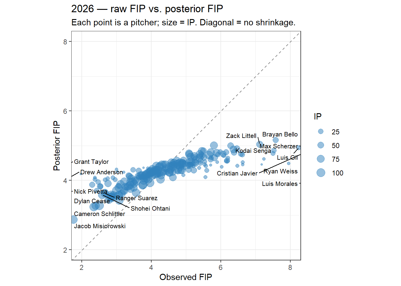
Low-IP pitchers (small dots) are pulled most strongly toward the diagonal. High-IP pitchers (large dots) are barely moved.
The plot below shows 80% credible intervals for the top starters by posterior WAR median.
season_scale <- min(
  1,
  (as.integer(max(d_logs$date) - min(d_logs$date)) + 1) / 186
)
ip_min_unc <- max(15L, round(50 * season_scale))

d_war |>
  filter(ip >= ip_min_unc) |>
  slice_head(n = 30) |>
  mutate(name = fct_reorder(name, war_med)) |>
  ggplot(aes(y = name, x = war_med)) +
  geom_vline(
    xintercept = 0,
    linewidth = 0.4,
    color = '#888888',
    lty = 'dashed'
  ) +
  geom_linerange(
    aes(xmin = war_lo, xmax = war_hi),
    linewidth = 0.7,
    color = '#3182bd',
    alpha = 0.7
  ) +
  geom_point(size = 2, color = '#3182bd') +
  scale_x_continuous(breaks = seq(-1, 8)) +
  labs(
    x = 'WAR',
    y = NULL,
    title = str_glue('{season} Pitcher WAR \u2014 Top 30 Starters'),
    subtitle = 'Points: posterior median  |  Bars: 80% credible interval'
  ) +
  theme_bw(base_size = 11) +
  theme(panel.grid.major.y = element_blank())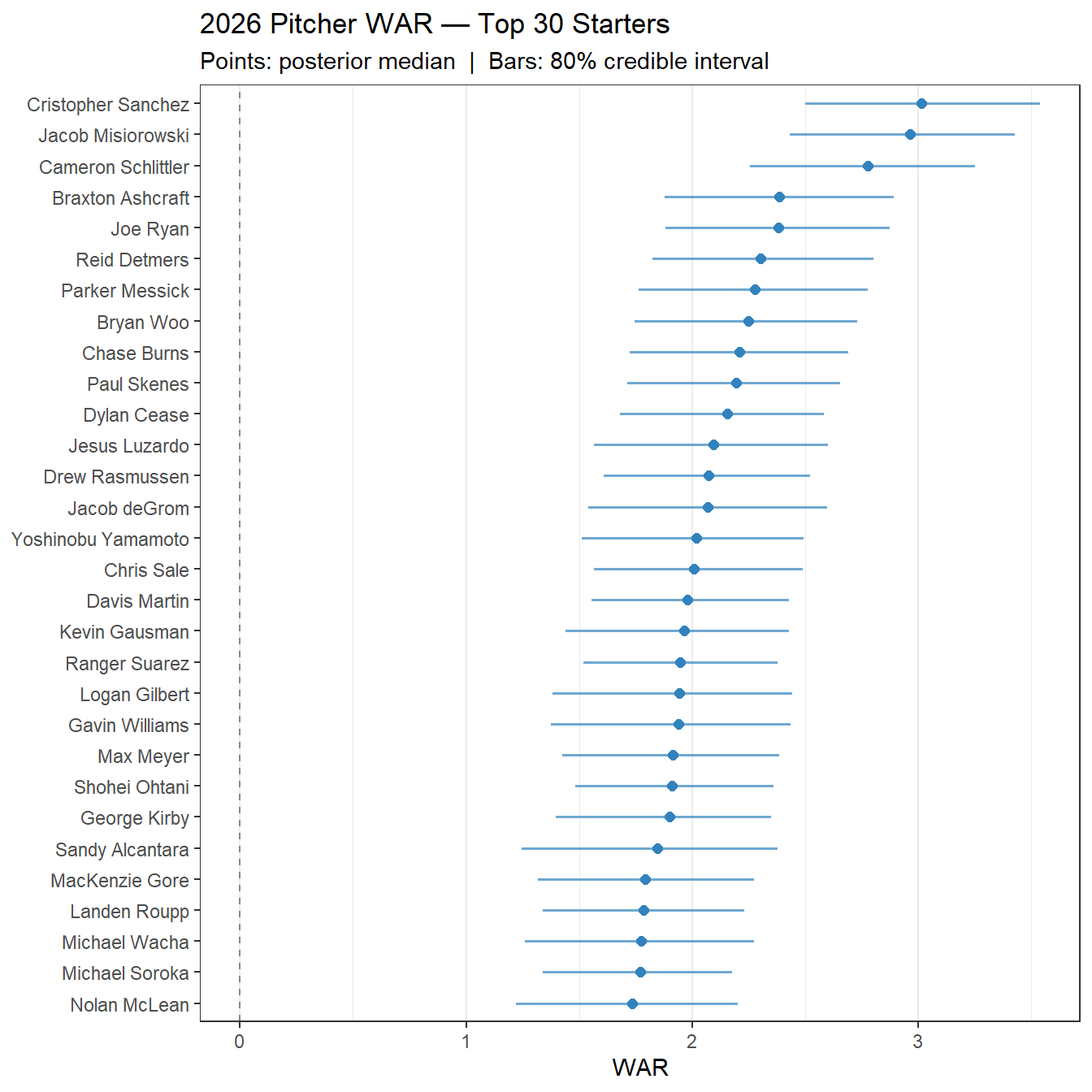
Interval widths narrow with innings pitched. A 200-IP ace has a tight estimate. A 50-IP pitcher’s WAR has real uncertainty even if the point estimate looks good.
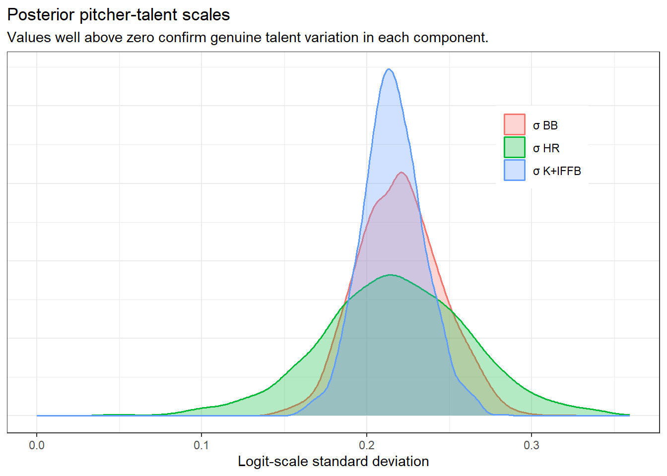
The \(\sigma_c\) parameters control how much pitcher-to-pitcher variation the model finds in each component. Posterior mass well away from zero confirms that genuine talent differences exist. A spike near zero would mean the model sees pitchers as essentially interchangeable for that component.
draws |>
  as_draws_df() |>
  select(sigma_k, sigma_bb, sigma_hr) |>
  pivot_longer(everything(), names_to = 'param', values_to = 'value') |>
  mutate(
    param = recode(
      param,
      sigma_k = '\u03c3 K+IFFB',
      sigma_bb = '\u03c3 BB',
      sigma_hr = '\u03c3 HR'
    )
  ) |>
  ggplot(aes(value, fill = param, color = param)) +
  geom_density(alpha = 0.3, linewidth = 0.7) +
  scale_x_continuous(limits = c(0, NA)) +
  labs(
    x = 'Logit-scale standard deviation',
    y = NULL,
    title = 'Posterior pitcher-talent scales',
    subtitle = 'Values well above zero confirm genuine talent variation in each component.',
    fill = NULL,
    color = NULL
  ) +
  theme_bw(base_size = 11) +
  theme(
    axis.text.y = element_blank(),
    axis.ticks.y = element_blank(),
    legend.position = 'inside',
    legend.position.inside = c(0.82, 0.75)
  )